|
Early in our optometric education, we all learned about aniseikonia and the equations for modifying ophthalmic lenses to compensate for perceived size differences. As full-fledged optometrists, we even think we know when it becomes clinically relevant. In school, we were taught how to differentiate between cases that could benefit from contact lenses vs. glasses based on keratometry readings and axial length measurements; we may have been shown a space eikonometer (though few of us have access to one in practice).
However, some literature calls into question many of the assumptions about aniseikonia we were taught as students.1 The research, as far back as 1999, demonstrates the flaws in assuming keratometry reading and axial length are key factors. Often, distortions in spatial perception trump the more purely optical considerations and must be tested directly and responded to, rather than being driven by the prescription alone. One of our recent cases reminded us of the importance of using those fundamental equations, not necessarily fancy technology, to solve the patient’s problems.
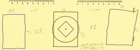 |
| Fig. 1. A patient’s cheiroscopic tracings show a significant size difference. Click image to enlarge. |
The Case
J.F., a current student at Southern College of Optometry, was undergoing vision therapy, but hit a wall as we attempted to build binocularity. Despite admirable compliance, he failed to make enough progress and saw little relief of his symptoms, including intermittent double vision, which he often closed an eye to avoid. He tilted his head to one side slightly, but was aware of it whenever he was fusing. He also experienced frequent headaches and asthenopia whenever he had to read for more than five to 10 minutes.
With the following prescription he could see 20/20+ with each eye:
• OD -0.25 -2.50 x 10⁸
• OS +1.50 -2.00 x 75
The difference in one meridian is about 1.75D and in the other meridian about 2.25D—this is hardly an amount that shouts
aniseikonia.
Student interns and residents repeatedly noted the presence of a large exophoria, which J.F. could converge to overcome, but fusion was just beyond reach. J.F. was experiencing significant near point symptoms, so we asked him to perform a cheiroscopic tracing. Using a stereoscope, we asked him to trace a picture presented in front of one occluded eye, using the other eye to help trace. Though the pencil point and picture are in different physical places, the patient perceives the pencil as tracing directly over the picture. We have the patient first perform this with the picture in front of the right eye, with the pencil tracing on the left of the recording paper. This is then repeated with the left eye with everything reversed.
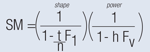 |
| Fig. 2. A colleague shared the spectacle magnification equation from his lecture notes. F1 is the front surface power of the lens, FV is the back vertex power, t is the lens thickness, n is the index of refraction and h is the distance from the lens’ back vertex to the entrance pupil. |
When J.F. performed the tracings, the figures were separated more than expected, in correlation with exophoria (Figure 1). The left tracing was lower than the central reference picture and the right one was shifted upward. This was consistent with the measured right hyperphoria. Another revelation: The left picture was about 7.6% narrower than the reference picture and the right tracing was about 8% wider—a possible explanation for J.F.’s fusion issues. We also noted that the right tracing looks twisted slightly in a clockwise direction but the floor of the tracing is nearly flat; the left tracing was not torqued at all. We tested for a cyclophoria using a subjective Double Maddox Rod test. It showed a three- to four-degree cyclophoria at distance. Generally, this is not perceived as a problem for the binocular system to overcome. However, a 7.6% to 8% perceptual size difference is often just at the point that it does cause a problem. We also noted the vertical size differences were not a big as the horizontal differences.
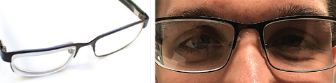 |
| Figs. 3 and 4. At left, J.F.’s lenses had significantly different thickness, yet they made a huge difference in his aniseikonia. At right, note the amount of the shift inwards of the right side of J.F.’s head in the temporal portion of his glasses and the lack of shift in the left side of his face. Click image to enlarge. |
Closing the Distance
The first approach was to get J.F. fit in contact lenses. He mentioned that he had been in and out of lenses and had a long-term problem with dry eye, which precludes his ability to wear contact lenses for any significant amount of time. Instead, it was time to break out the equations to compute a new set of spectacles for J.F. (Figure 2).
To make things a little more convenient, we used a calculation tool at opticampus.com (64.50.176.246/tools/magnification.php). Putting this formula into practice prompted a phone call to our lab to clarify a few parameters:
• What is a practical range of front base curves to which we can have lenses ground?
• What is the practical thickest lens you could accommodate?
The practical base curve range was from +0.50 to +8.00, and the thickest lens we’d explore would have a 6mm center thickness.
When we put J.F.’s current glasses Rx into the equation, we saw they were producing about 3% of the 7.6% to 8% size difference noted by the tracing. His original glasses were done on a +3.50 front surface base curve.
We then explored a range of lenses and materials to come up with the following Rx:
• OD -0.25 -2.50 x 10⁸ with a +8.00 base curve and 6.0mm center thickness.
• OS +1.50 -2.00 x 75 with a +0.50 base curve and a 2.2mm center thickness.
This achieved a 2.8% increase in the size of the right eye image and a 0.5% decrease in size in the left eye for a net 3.3% decrease in size difference (Figures 3 and 4). We hoped it would be enough.
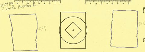 |
| Fig. 5. J.F.’s second tracing showed significantly less difference in size. Click image to enlarge. |
The Difference is Clear
After wearing the new glasses for about 25 minutes, J.F. completed a second cheiroscopic tracing (Figure 5). The horizontal size in the right tracing matched the reference figure. The left tracing was less stable, as the top was wider and the bottom was narrower than the reference. Also, the figures are a bit closer to the center and the vertical deviation is somewhat reduced (Figure 5).
Did the new prescription make a difference? J.F. wrote the next morning, “Usually, I end up closing my left eye reading my scriptures in the morning. I was able to comfortably read with both eyes open with the new glasses on. Woohoo!”
Oh, and these lenses only cost $38.85.
As J.F. reminded us, we can diagnose and treat aniseikonia without the need for a space eikonometer; treatment need not cost a fortune, nor do we need to fall prey to expensive proprietary systems to address the clinical problems. Sometimes, in ophthalmic prescribing, size differences do matter.
| 1. Romano PE, Von Noorden GL. Knapp’s law and unilateral axial high myopia. Bin Vis Strab Quart. 1999;14:215-22. |