|
In June 2012, a 57-year-old Caucasian female presented to the office with complaints related to headaches and periocular discomfort that progressed over several months. She was a low hyperope wearing a hyperopic presbyopic spectacle prescription that was about five years old at the time.
She was taking no medications and reported no allergies to medications. Refractively, she had an expected change in her spectacle prescription of increased hyperopia and presbyopia, best corrected to 20/20 OD, OS, OU.
A slit lamp exam of her anterior segments was unremarkable. Applanation tensions at that visit were 15mm Hg OD and OS at 10:39am. Slit lamp estimation of her anterior chamber angles demonstrated wide-open angles in both eyes.
Through dilated pupils, her crystalline lenses were clear bilaterally. Her cup-to-disc ratios were 0.65 x 0.75 OD and 0.65 x 0.65 OS, with discs that were average size. There was slight thinning of the temporal rim in both eyes, with a common appearance of sloping temporal margins of the neuroretinal rim into the optic cup. Her macular, vascular and retinal evaluations were normal in both eyes.
I asked her if anyone had mentioned that she had some characteristics to her optic nerves that put her at risk for glaucoma, and she said no. She also denied a family history of glaucoma. I explained my findings of suspicious discs and, since she was dilated, I took the opportunity to obtain stereo optic nerve images. She was scheduled for a full glaucoma work-up in the next few weeks.
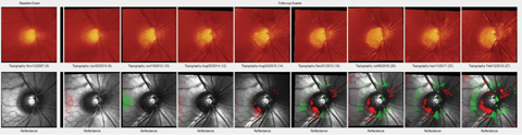 |
| HRT 3 imaging shows a distinct change in the IT neuroretinal rim of our patient’s right eye, first noted in 2015. Click image to enlarge. |
Evaluation
As scheduled, she presented for the glaucoma work-up, which included pachymetry, morning IOP readings, gonioscopy, threshold visual fields and Heidelberg retina tomograph (HRT 3) and optical coherence tomography (OCT) imaging of the optic nerves. At this visit, pachymetry readings were 478µm OD and 479µm OS. Applanation tensions at 9:15am were 16mm Hg OD and 17mm Hg OS. Gonioscopy demonstrated wide-open angles with minimal trabecular pigmentation, a flat iris-to-angle approach and no angle abnormalities. Threshold standard automated perimetry (SAP) field studies were clear and reliable in both eyes. HRT 3 nerve imaging confirmed the clinical appearance of the optic nerves with a large cup, a thinned temporal neuroretinal rim and Moorfields Regression Classification as statistically borderline optic nerves in both eyes. The RNFL circle scan of both eyes was statistically normal.
Given the findings at that time, I diagnosed her as a glaucoma suspect only, as there was no frank evidence of glaucoma either structurally or functionally. I asked her to follow up in a year.
Over the subsequent years, she presented annually as directed, and essentially all findings remained stable, though we did substitute threshold flicker-defined form visual fields for SAP fields, looking specifically for early field loss. These too remained stable. However, in the summer of 2015, there appeared to be a change in the inferotemporal neuroretinal rim of the OD from baseline, while all other indices remained stable. Given that her imaging to this point was stable and consisted of high quality images, this change was worthy of further investigation. Accordingly, I asked her to return in four months for repeat nerve imaging. At that visit in December 2015, the structural defect had worsened in the right eye, indicating a conversion to early glaucoma. Her imaging of the left eye remained stable insofar as the HRT 3 images were concerned. And her OCT RNFL circle scans also remained stable.
Accordingly, she was initially managed with 0.5% timolol QAM to the right eye, and observation of the left eye. Post treatment IOP readings in the right eye have averaged 11mm Hg to 12mm Hg, and those of the unmedicated the left eye have remained in the mid-teen range.
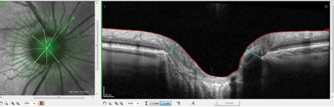 |
| This radial OCT image of the right eye shows a commonly seen steep nasal margin and a more sloping inferotemporal margin. Click images to enlarge. |
Discussion
Once the patient converts from a glaucoma suspect to a patient needing intervention, I usually see them a bit more frequently, and as such, I followed the same protocol with this patient. At this point in our management, each visit is tasked with determining whether the patient remains stable or not, which, for glaucoma, requires an evaluation of both the structural and functional aspects of the eye.
One of the advantages of having adequate instrumentation to evaluate these patients is that one can see, rather readily, when it occurs, change over time. One of the disadvantages to having a variety of ways to evaluate stability over time is that sometimes the quantity of information becomes overwhelming. With too much data in our hands, it’s easy to see situations where busy clinicians might not evaluate all of the pieces to the diagnostic puzzle and miss significant changes.
So how much technology is too much? And how much is too little? Those answers are going to vary from practice to practice, and there are no concrete answers I can give to you. But this case highlights why having multiple technologies can help you to offer personalized care, if you take the time to sift through the date. The radial OCT image on page 89 shows one of the more common presentations of an optic nerve with temporal sloping margins, especially in the IT sector where the HRT 3 image was showing changes.
When we look at OCTs of change, we can look at several locations. Most optometrists probably first look at the perioptic RNFL circle scan. Now that we are scanning several different diameter RNFL circle scans, we can detect changes that are occurring at various distances from the optic nerve, and not just the standard 3.5mm circle scan.
Finally, peeling back even more detail, we can take a look specifically at the IT sector of the OCT Bruch’s membrane opening (BMO) map for change. Given the ability to now look at BMO in various sectors of the optic nerve, and the statistical capability of looking for change over time in these individual sectors, we can now look at not only the macular and perioptic RNFL areas, but also at the neuroretinal rim. Remember, in this case, she showed signs of conversion in the IT sector of the neuroretinal rim as seen on the HRT 3. This same sector, as seen on the BMO OCT scan, over two visits, shows complete stability.
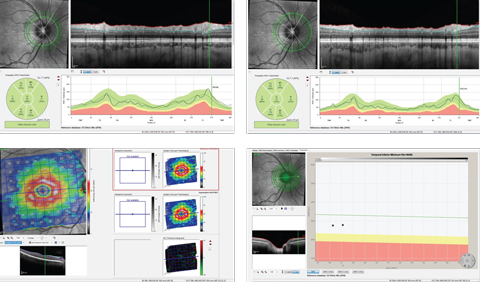 |
| Top row, temporal-superior-nasal-inferior-temporal RNFL circle scans of two different diameters, with the top right image showing the circle scan obtained at a 4.7mm diameter scan. Bottom row left, this macular ganglion cell layer thickness change map of the patients right eye shows stability. Bottom right, this IT BMO OCT scan with minimum rim shows stability over time. Click images to enlarge. |
Changes
The key diagnostic piece to this puzzle is that the initial change occurred in the IT sector of the OD, as measured by one instrument. Subsequent measurements of the same sector of the neuroretinal rim with a different instrument (OCT) show no change. And it is in this area where she would most likely show continued progression if it occurred.
Instruments change. Technology changes. Optic nerves change, if they are worsening. Knowing where to look is half the battle. Looking through all the data, though challenging, is what makes for excellent clinical care.